
From below I’ve quoted some paragraphs from page 59~page 70 directly in the ISLR book.
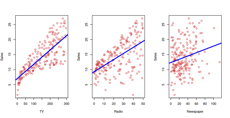
Recall the Advertising data from Chapter 2. The figure below displays sales for a particular product as a function of advertising budgets for TV, radio, and newspaper media. Suppose that in our role as statistical consultants we are asked to suggest, on the basis of this data, a marketing plan for next year that will result in high product sales. What information would be useful in order to provide such a recommendation? Here are a few important questions that we might seek to address:
- Is there a relationship between advertising budget and sales?
- How strong is the relationship between advertising and sales?
- Which media contribute to sales?
- How accurately can we estimate the effect of each medium on sales?
- How accurately can we predict future sales?
- Is the relationship linear?
- Is there synergy among the advertising media?
3.1 Simple Linear Regression
It is a very straightforward approach for predicting a quantitative response Y on the basis of a single predictor variable X. It assumes that there is approximately a linear relationship between X and Y. Mathematically, we can write this linear relationship as
Y\approx \beta_0 + \beta_1X
\beta_0 and \beta_1 are two unknown constants that represent the intercept and slope terms in the linear model. Together, \beta_0 and \beta_1 are known as coefficients or parameters. Once we have used our training data to produce estimates \hat{\beta_0} and \hat{\beta_1} for the model coefficients, we can predict future sales on the basis of a particular value of TV advertising by computing
\hat{y}=\hat{\beta_0}+\hat{\beta_1}x
3.1.1 Estimating the Coefficients
Let (x_1, y_1), (x_2, y_2), ..., (x_n, y_n)
represent n observations pairs, each of which consists of a measurement of X and a measurement of Y.
Let \hat{y_i}=\hat{\beta_0}+\hat{\beta_1}x_i be the prediction for Y based on the i th value of X. Then e_i = y_i - \hat{y_i} represents the i th residual-this is the difference between the i th observed response value and the i th response value that is predicted by our linear model. We define residual sum of squares (RSS) as
RSS = e_1^2 + e_2^2 + \cdots + e_n^2
The least square approach chooses \hat{\beta_0} and \hat{\beta_1} to minimize the RSS. Using some calculation, one can show that the minimizers are
\hat{\beta_1}= \dfrac{\sum^n_{i=1}(x_i-\bar{x})(y_i-\bar{y})}{\sum^n_{i=1}(x_i-\bar{x})^2}
\hat{\beta_0}=\bar{y}-\hat{\beta_1}\bar{x} —– (3.4)
3.1.2 Assessing the Accuracy of the Coefficient Estimates
population regression line : Y = \beta_0 + \beta_1X + \epsilon
, where~ \epsilon mean zero random error term
least squares line : \hat{y}=\hat{\beta_0}+\hat{\beta_1}x
(true relationship between X and Y takes the form Y=f(X)+\epsilon)
Fundamentally, the concept of these two lines (population regression line vs. least squares line) is a natural extension of the standard statistical approach of using information from a sample to estimate characteristics of a large population. For example, suppose that we are interested in knowing the population mean \mu of some random variable Y. Unfortunately, \mu is unknown, but we do have access to n observations from Y, which we can write as y_1, y_2, \cdots, y_n , and which we can use to estimate \mu . A reasonable estimate is \hat{\mu} = \hat{y} , where \hat{y} = \dfrac {1}{n}\sum^n_{i=1}{y_i} is the sample mean. The sample mean and the population mean are different, but in general the sample mean will provide a good estimate of the population mean. In the same way, the unknown coefficients \beta_0 and \beta_1 in linear regression define the population regression line. We seek to estimate these unknown coefficients using \hat{\beta_0} and \hat{\beta_1} given in (3.4). These coefficient estimates define the least squares line.
The analogy between linear regression and estimation of the mean of a random variable is an apt one based on the concept of bias. If we use the sample mean \hat{\mu} to estimate \mu , this estimate is unbiased, in the sense that on average, we expect \hat{\mu} to equal \mu . What exactly does this mean? It means that on the basis of one particular set of observations y_1, y_2, \cdots, y_n , \hat{\mu} might overestimate \mu , and on the basis of another set of observations, \hat{\mu} might underestimate \mu . But if we could average a huge number of estimates of \mu obtained from a huge number of sets of observations, then this average would exactly equal \mu . Hence, an unbiased estimator does not systematically over- or under-estimate the true parameter. The property of unbiasedness holds for the least squares coefficient estimates given by (3.4) as well: if we estimate \beta_0 and \beta_1 on the basis of a particular data set, then our estimates won’t be exactly equal to \beta_0 and \beta_1 . But if we could average the estimates obtained over a huge number of data sets, then the average of these estimates would be spot on! In fact, we can see from the right-hand panel of Figure 3.3 that the average of many least squares lines, each estimated from a separate data set, is pretty close to the true population regression line.
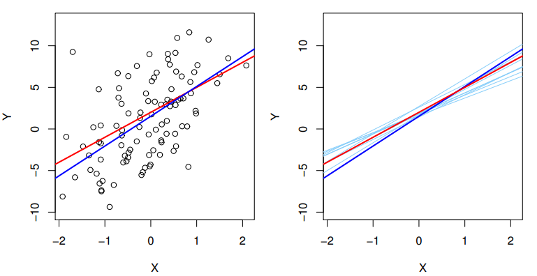 Figure 3.3 A simulated data set. Left: The red line represents the true relationship, f(X) = 2+3X , which is known as the population regression line. The blue line is the least squares line; it is the least squares estimate for f(X) based on the observed data, shown in black. Right: The population regression line is again shown in red, and the least squares line in dark blue. In light blue, ten least squares lines are shown, each computed on the basis of a separate random set of observations. Each least squares line is different, but on average, the least squares lines are quite close to the population regression line.
We continue the analogy with the estimation of the population mean \mu of a random variable Y. A natural question is as follows: how accurate is the sample mean \hat{\mu} as an estimate of \mu ? We have established that the average of \hat{\mu} ‘s over many data sets will be very close to \mu , but that a single estimate \hat{\mu} may be a substantial underestimate or overestimate of \mu . How far off will that single estimate of \hat{\mu} be? In general, we answer this question by computing the standard error of \hat{\mu}, written as SE(\hat{\mu}). We have the well-known formula
Var(\hat{\mu})=SE(\hat{\mu})^2=\dfrac{\sigma^2}{n} —- (3.7)
,where \sigma is the standard deviation of each of the realization y_i of Y. (This formula hold provided that the n observations are uncorrelated.)
Roughly speaking, the standard error tells us the average amount that this estimate \hat{\mu} differs from the actual value of \mu . Equation 3.7 also tells us how thie deviation shrinks with n–the more observations we have, the smaller the standard error of \hat{\mu} . In a simillar vein, we can wonder how close \hat{\beta_0} and \hat{\beta_1} are to the true values \beta_0 and \beta_1 . To compute the standard errors associated with \hat{\beta_0} and \hat{\beta_1} , we use the following formulas:
SE(\hat{\beta_0})^2 = \sigma^2[\dfrac{1}{n}+\dfrac{\bar{x}^2}{\sum^n_{i=1}{(x_i-\bar{x})^2}}],~~~SE(\beta_1)^2=\dfrac{\sigma^2}{\sum^n_{i=1}(x_i-\bar{x})^2}
,where \sigma^2=Var(\epsilon) .
For these formulas to be strictly valid, we need to assume that the errors \epsilon_i for each observations are uncorrelated with common variance \sigma^2 . This is clearly not true in Figure 3.1, but the formula that SE(\hat{\beta_1}) is smaller than when the x_i are more spread out; intuitively we have more leverage to estimate a slope when this is the case. We also see that SE(\hat{\beta_0}) would be the same as SE(\hat{\mu}) if \bar{x} were zero (in which case \hat{\beta_0} would be equal to \hat{y} ).
In general, \sigma is not known, but can be estimated from the data. This estimate is known as the residual standard error, and is given by the formula RSE = \sqrt{RSS/(n-2)} . Strictly speaking, when \sigma^2 is estimated from the data we should write \widehat{SE}(\hat{\beta_1}) to indicate that an estimate has been made, but for simplicity of notation we will drop this extra “hat”.
Standard errors can be used to compute confidence intervals. A 95% confidence interval is defined as a range of values such that with 95% probability, the range will contain the true unknown value of the parameter. The range is defined in terms of lower and upper limits computed from the sample of data. For linear regression, the 95% confidence interval for \beta_1 approximately takes the form
\hat{\beta_1}\pm2\cdot SE(\hat{\beta_1})
That is, there is approximately a 95% change that the interval
[\hat{\beta_1}-2\cdot SE(\hat{\beta_1}),~\hat{\beta_1}+2\cdot SE(\hat{\beta_1})]
will contain the true value of \hat{\beta_1} . Similarly, a confidence interval for \beta_0 approximately takes the form
\hat{\beta_0}\pm2\cdot SE(\hat{\beta_0})
◎ Hypothesis Tests
Standard errors can also be used to perform hypothesis tests on the coefficients. The most common hypothesis test involves testing the null hypothesis of
H_0 : There is no relationship between X and Y
versus the alternative hypothesis
H_a : There is some relationship between X and Y
Mathematically, this corresponds to testing
H_0 : \beta_1 = 0H_a : \beta_1 \not = 0
since if \beta_1 = 0 then the model reduces to Y=\beta_0+\epsilon , and X is not associated with Y. To test the null hypothesis, we need to determin whether \hat{\beta_1} , our estimate for \beta_1 , is sufficiently far from zero that we can be confident that [\beta_1] is non-zero. How far is far enough? This is course depends on the accuracy of \hat{\beta_1} -that is, it depends on SE(\hat{\beta_1}) . If SE(\hat{\beta_1}) is small, then even relatively small values of \hat{\beta_1} may provide strong evidence that \beta_1 \not = 0 , and hence that there is a relationship between X and Y. In contrast, if SE(\hat{\beta_1}) is large, then \hat{\beta_1} must be large in absolute value in order for us to reject the null hypothesis. In practice, we compute a t-statistic, given by
t=\dfrac{\hat{\beta_1}-0}{SE(\hat{\beta_1})} —– (3.14)
(3.14) will have a t-distribution with n-2 degrees of freedom. The t-distribution has a bell shape and for values of n greater than approximately 30 it is quite similar to the normal distribution. Consequently, it is a simple matter to compute probability of observing any value equal to |t| or larger, assuming \beta_1 =0 . We call this probability the p-value.
P(|T| > t) = p
Roughly speaking, we interpret the p-value as follows: a small p-value indicates that it is unlikely to observe such a substantial association between the predictor and the response due to chance, in the absence of any real association between the predictor and the response. Hence, if we see a small p-value, then we can infer that there is an association between the predictor and the response.We reject the null hypothesis-that is, we declare a relationship to exist between X and Y- if the p-value is small enough.Typical p-value cutoffs for rejecting the null hypothesis are 5 or 1 %. When n = 30, these corresponds to t-statistics of around 2 and 2.75, respectively.
3.1.3 Assessing the Accuracy of the Model
① Residual Standard Error (RSE) :
Recall from the model (3.5) – Y=\beta_0+\beta_1X+\epsilon – that associated with each observation is an error term \epsilon . Due to the presence of these error terms, even if we knew the true regression line, we would not be able to perfectly predict Y from X. The RSE is an estimate of the standard deviation of \epsilon . Roughly speaking, it is the average amount that the response will deviate from the true regression line. It is computed using the formula
Note the RSS was defined in Section 3.1.1, and is given by the formula
RSS = \sum^n_{i=1}(y_i-\hat{y_i})^2 —- (3.16)
② R^2 Statistic :
RSE provides and absolute measure of lack of fit of the model (3.5) to the data. The R^2 statistic provides an alternative measure of fit. It takes the form of a proportion-the proportion of variance explained-and so it always takes on a value between 0 and 1, and is independent of the scale of Y. To calculate R^2 , we use the formula
R^2=\dfrac{TSS-RSS}{TSS}=1-\dfrac{RSS}{TSS} —- (3.17)
,where TSS =\sum{y_i-\bar{y}}^2 is the total sum of squares, and RSS is defined in (3.16). TSS measures the total variance in the response Y, and can be thought of as the amount of variability inherent in the response before the regression is performed. In contrasts, RSS measures the amount of variability that is left unexplained after performing the regression. Hence, TSS – RSS measures the amount of variability in the response that is explained (or removed) by performing the regression, and R^2 measures the proportion of variability in Y that can be explained using X. An R^2 statistic that is close to 1 indicates that a large proportion of the variability in the response has been explained by the regression.
The R^2 statistic has an interpretational advantage over the RSE (3.15), since unlike the RSE, it always lies between 0 and 1. However, it can still be challenging to determine what is a good R^2 value, and in general, this will depend on the application. For instance, in certain problems in physics, we may know that the data truly comes from a linear model with a small residual error. In this case, we would expect to see an R^2 value that is extremely close to 1, and a substantially smaller R^2 value might indicate a serious problem with the experiment in which the data were generated. On the other hand, in typical applications in biology, psychology, marketing, and other domains, the linear model (3.5) is at best an extremely rough approximation to the data, and residual errors due to other unmeasured factors are often very large. In this setting, we would expect only a very small proportion of the variance in the response to be explained by the predictor, and an R^2 value well below 0.1 might be more realistic!
The R^2 statistic is a measure of the linear relationship between X and Y. Recall that correlation, defined as
Cor(X, Y)=\dfrac{\sum^n_{i=1}(x_i-\bar{x})(y_i-\bar{y})}{\sqrt{\sum^n_{i=1}(x_i-\bar{x})^2}\sqrt{\sum^n_{i=1}(y_i-\bar{y})^2}}
is also a measure of the linear relationship between X and Y. This suggests that we might be able to use r=Cor(X,Y) instead of R^2 in order to assess the fit of the linear model. In fact, it can be shown that in the simple linear regression setting, R^2=r^2 .